Price 3.0
From Evolution and Games
(→The Price equation for this very simple model) |
|||
| Line 1: | Line 1: | ||
[[Category:Price equation]] | [[Category:Price equation]] | ||
| + | [[Price | Go to the front-page of Price equation tutorials ]] | ||
| + | |||
== A model with frequency dependence == | == A model with frequency dependence == | ||
Revision as of 22:39, 18 September 2010
Go to the front-page of Price equation tutorials
A model with frequency dependence
We go back to the asexual model, but now we will take a model with frequency dependence. This will be a bit more complicated, but we can still use a basic, well known model. Suppose there are $N$ individuals. They are paired randomly, and play a game in those pairs. The game gives them payoffs according to the following payoff matrix

If qi = 1, then that means that individual $i$ plays strategy A, and qi = 0 means that individual i plays strategy B. Depending on the match, each individual gets a payoff πi. The next generation is drawn, as before, one individual at a time. But now the probability that i is drawn as a parent depends on the payoff, and not just on the own genotype.
We do the same procedure as before, but with a few different starting points.
An A mutant in a population of B's
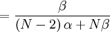
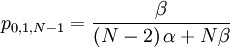
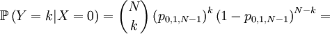
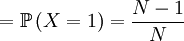
Suppose q1 = 1 and qi = 0 for i = 2,...,N. The probability of any individual i = 2,...,N to be matched with individual 1 is 1 / (N − 1).
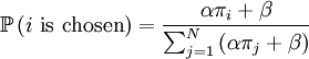
The probability with which an individual i with qi = 1, who is matched to an individual j with qj = 0, is chosen is:
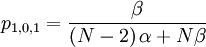
The probability with which an individual i with qi = 0, who is matched to an individual j with qj = 0, is chosen is:
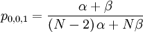
The probability with which an individual i with qi = 0, who is matched to an individual j with qj = 1, is chosen is:
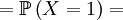
We can also compute the covariance of these two actual random variables. Let us start by computing expectations...
![\mathbb{E}\left[ X\right] =\frac{1}{N}](/wiki/images/math/c/3/8/c389f3bfffa4dec33da0820781e6e99b.png)
![\mathbb{E}\left[ X\right] =\sum_{x=0,1}x\mathbb{P}\left( X=x\right) =](/wiki/images/math/5/c/8/5c8589cd4e69154ab8f56f7db9f0dc8f.png)

For symmetry reasons...
![\mathbb{E}\left[ Y\right] =1](/wiki/images/math/f/6/8/f6851309af9717e71df00c1227f0d760.png)
![\mathbb{E}\left[ XY\right] =\frac{\beta }{\left( N-2\right) \alpha +N\beta }](/wiki/images/math/b/c/1/bc1ba1eb3290d07e011aad2aaf8c6036.png)
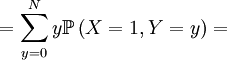
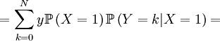
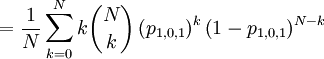
![\mathbb{E}\left[ XY\right] =\sum_{x=0,1}\sum_{y=0}^{N}xy\mathbb{P}\left(X=x,Y=y\right) \text{ (because }xy=0\text{ if either }x=0\text{ or }y=0\text{)}](/wiki/images/math/f/1/4/f146e34f77cefe890894be133473bf2a.png)
The Covariance is thus...
![Cov\left( X,Y\right) =\mathbb{E}\left[ XY\right] -\mathbb{E}\left[ X\right] \mathbb{E}\left[ Y\right] =\frac{\beta }{\left( N-2\right) \alpha +N\beta }-\frac{1}{N}](/wiki/images/math/4/5/1/451efdc1824fac07a0b1bf56a8167a29.png)
A B mutant in a population of A's
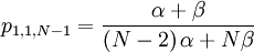
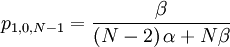
Suppose q1 = 0 and qi = 1 for i = 2,...,N. The probability of any individual i = 2,...,N to be matched with individual 1 is 1 / (N − 1).
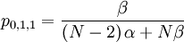
The probability with which an individual i with qi = 0, who is matched to an individual j with qj = 1...
The probability with which an individual i with qi = 1, who is matched to an individual j with qj = 1...
The probability with which an individual i with qi = 1, who is matched to an individual j with qj = 0...
So...

This is pretty well defined, so we can also compute the covariance of these two actual random variables. Let us start with the expectations...
![\mathbb{E}\left[ X\right] =\frac{N-1}{N}](/wiki/images/math/8/a/9/8a9d1397815d5042bde4b9407714f7da.png)
For symmetry reasons...
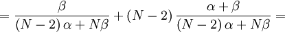
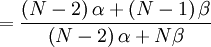
![\mathbb{E}\left[ XY\right] = \frac{\left( N-2\right) \alpha +\left( N-1\right) \beta }{\left(N-2\right) \alpha +N\beta }](/wiki/images/math/a/1/b/a1b3f65cc47eb865d7eaed9b55f193af.png)
![=\frac{N-1}{N}\sum_{k=0}^{N}\left[ \frac{1}{N-1}k\binom{N}{k}\left(p_{1,0,N-1}\right) ^{k}\left( 1-p_{1,0,N-1}\right) ^{N-k}+\frac{N-2}{N-1}k\binom{N}{k}\left( p_{1,1,N-1}\right) ^{k}\left( 1-p_{1,1,N-1}\right) ^{N-k}\right]](/wiki/images/math/7/4/9/749b567e6d87135a52d34cb2787efab1.png)

Thus....
![Cov\left( X,Y\right) =\mathbb{E}\left[ XY\right] -\mathbb{E}\left[ X\right] \mathbb{E}\left[ Y\right] =\frac{\left( N-2\right) \alpha +\left( N-1\right)\beta }{\left( N-2\right) \alpha +N\beta }-\frac{N-1}{N}](/wiki/images/math/a/f/e/afe717cf465e229083a9af7442bd1559.png)
Comparing the two covariances
If we compare these two covariances, for instance for β = 0 and α = 1, then in the first case Cov(X,Y) = − 1 / N, while in the second case Cov(X,Y) = + 1 / N. This should not feel strange; it is a coordination game, and if everyone plays B, then playing A is a bad idea, but if everyone else plays A too, then playing A is a good idea. The model covariance is therefore not constant, and changes with the frequency of strategy A.
The Price equation for this very simple model
Here we have a nested sampling procedure; you can choose a starting point (by clicking on each individual in the parent population), keep it fixed, and draw a few transitions. Then change your starting point, and draw a few transitions from there. You will notice that the Price equation varies with every transition, along with the likelyhood of the different transitions that depend on the initial population.
What would a proper probability theorist do?
Try to figure out the transition probabilities for the suggested model as a function of the current state. It seems that Nowak, Liebermann, Ohtsuki and Tarnita are a proper probability theorists, because that is what they did already.
What would a proper statistician do?
Sample often for different starting points. Fit data to the model, estimate α and β. Test if the payoff matrix is as assumed.
So how does the Price equation help here?
Not. Can't think of anything remotely useful about the Price equation. The extra problem here is the frequency dependence. Sometimes this is referred to as the problem that the Price Equation is not dynamically sufficient. That is a step in the right direction, but still inaccurate, because it only describes one of the symptoms, and not the cause. It is the model we have here that gives us, after a bit of computing, the transition probabilities for all frequencies of A, and thereby all properties of the dynamical system. The models in versions 1.0 and 2.0 just concerned transitions leaving from one given starting point. A model can therefore be described as dynamically sufficient or insufficient. Because the Price equation can only deal with one step at at time, it tends to inspire people to think of implicit assumptions that pertain to dynamically insufficient models. That, however, does not mean that the Price Equation cannot be used in combination with a dynamically sufficient model. It can; as shown in the applet above. But the question is: used for what? And the answer is: for nothing.
