Price 1.0

From Evolution and Games

Revision as of 07:25, 18 September 2010 (view source) Julian.garcia (Talk | contribs) (→Intro) ← Older edit		Revision as of 07:34, 18 September 2010 (view source) Julian.garcia (Talk | contribs) (→Intro) Newer edit →
Line 41:		Line 41:
	<math>Cov\left( X,Y\right) =\mathbb{E}\left[ XY\right] -\mathbb{E}\left[ X\right]		<math>Cov\left( X,Y\right) =\mathbb{E}\left[ XY\right] -\mathbb{E}\left[ X\right]
	\mathbb{E}\left[ Y\right] =p-\frac{1}{2}\cdot 1=p-\frac{1}{2} </math>		\mathbb{E}\left[ Y\right] =p-\frac{1}{2}\cdot 1=p-\frac{1}{2} </math>
		+
		+	<toggledisplay>
		+
		+	<math>\mathbb{E}\left[ XY\right] =\sum_{x=0,1}\sum_{y=0,1,2}xy\mathbb{P}\left( X=x,Y=y\right)  </math>
		+
		+	(because <math>xy=0</math> if either <math>x=0</math> or <math>y=0</math>
		+
		+	<math> =\sum_{x=1}\sum_{y=1,2}xy\mathbb{P}\left( X=x,Y=y\right) = </math>
		+
		+	<math> =1\cdot \mathbb{P}\left( X=1,Y=1\right) +2\cdot \mathbb{P}\left(X=1,Y=2\right) = </math>
		+
		+	<math> =1\cdot \mathbb{P}\left( X=1\right) \cdot \mathbb{P}\left(Y=1|X=1\right) +2\cdot \mathbb{P}\left( X=1\right) \mathbb{P}\left(Y=2|X=1\right) = </math>
		+
		+	<math> =1\cdot \frac{1}{2}\cdot 2p\left( 1-p\right) +2\cdot \frac{1}{2}\cdot p^{2}= </math>
		+
		+	<math>=p\left( 1-p\right) +p^{2}= </math>
		+
		+	<math> =p</math>
		+
		+
		+
		+
		+
		+
		+
		+
		+	</toggledisplay>

---

Revision as of 07:34, 18 September 2010

Intro

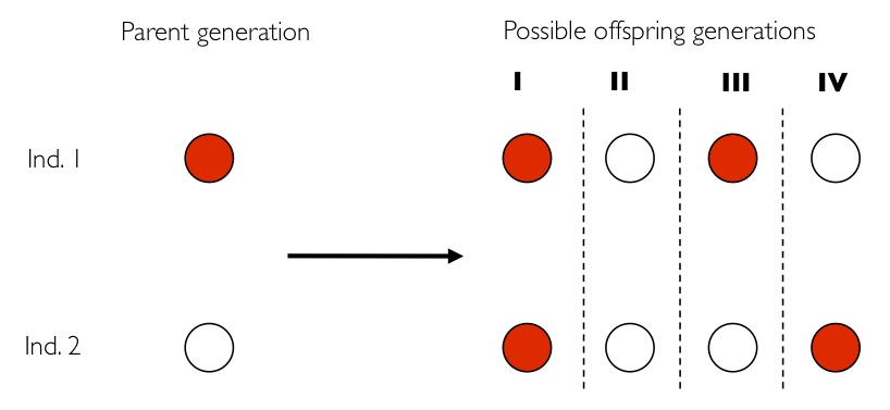
Suppose that we have a population of 2 individuals. We depart from a population in which individual no 1 has "the" gene, while the other, individual no 2, does not. In Price equation terms, that means that the variable q_i, which denotes the frequency of the gene in individual i becomes: q₁ = 1, q₂ = 0.

The next generation of 2 individuals is drawn in a very simple way. First we draw the first, and then we draw the second. That makes it - for those who care - a Wright-Fisher process. At both draws the new individual could be the offspring of individual no 1 or of individual no 2. Reproduction is asexual, hence the offspring is a perfect copy of its parent. Now here comes the important thing. We assume that at both draws, the probability of no 1 from the parent population -- the one with the gene -- to be drawn for reproduction is p, while the probability of no 2 from the parent population -- the one without the gene -- to be drawn for reproduction is 1 − p. That gives us four possible transitions.

What the new generation will be is a random variable. What the current generation is, is not; the current generation is simply given. We can however think of a hypothetical chance experiment such that, in combination with the actual random transition, we get two random variables, between which we can define a covariance. So here is the recipe.

1) Draw one of the individuals from the parent population (this is the hypothetical random variable).

2) Draw the next generation (this is the actual random thing that happens in the the transition).

The random variable X is now defined as the genotype of the parent. That is a simple, albeit hypothetical random variable:

.

Then we define the random variable Y, which is the number of offspring that the parent that has been drawn begets. This is a slightly more complicated random variable, because the chances depend on which of the two the (candidate) parent is. So we get a (not too long) list of conditional probabilities. Worth working through!

Because the parent of a new individual is the one if it is not the other, and vice versa, the other conditional probabilities are the reverse.

The X and Y are pretty well defined, so we can also compute the covariance of these two actual random variables. There we go:

[show details]