Sociality
From Evolution and Games
This page is under construction, in the meantime please go here.
The software we provide and describe here reimplements simulations first described in Aviles 2002 using Java . Our simulation program also has alternative fitness functions and some additional features. If you have questions or require further information about this work or this tutorial please do email Julian Garcia, Matthijs van Veelen or Leticia Avilés.
Contents |
Editorial Information
van Veelen, Matthijs, García Julián and Avilés Leticia (in Press). It takes grouping and cooperation to get sociality. Journal of Theoretical Biology.
Abstract
Cooperation and grouping are regularly studied as separate traits. The evolution of sociality however requires both that individuals get together in groups and that they cooperate within them. Because the level of cooperation can influence selection for group size, and vice versa, it is worth studying how these traits coevolve. Using a generally applicable two-trait optimization approach, we provide analytical solutions for three specific models. These solutions describe how cooperative associations of nonrelatives evolve, and predict how large and how cooperative they will be. The analytical solutions help understand how changes in parameter values, such as the group carrying capacity and the costs of cooperation, affect group size and the level of cooperation in equilibrium. Although the analytical model makes a few simplifying assumptions - populations are assumed to be monomorphic for grouping as well as for cooperative tendencies, and group size is assumed to be deterministic - simulations show that its predictions are matched quite closely by results for settings where these assumptions do not hold.
Run the simulations
The genetic system
What individuals are made of
Individuals are characterized by a diploid genome coding for two separate traits; grouping and cooperative tendencies. The number of loci for each of these traits can be chosen by the user of the program. The number of loci for grouping will be denoted by n, and the number of loci for cooperation will be denoted by m. We followed Avilés et al. (2002) by choosing 15 as a default value for the number of loci for both traits. The loci of an individual will be numbered from 1 to n + m, where the first n loci code for grouping tendencies and the loci from n+1 to n+m code for cooperative tendencies. The alleles will be indicated as left and right. At each locus, two alleles (1 or 0) can occur. The tendency of individual i to form groups is denoted by gi, and equals the proportion of 1’s in the grouping portion of its genome, or the number of 1’s divided by 2n. The tendency of individual i to cooperate, denoted by Íi, is the proportion of 1’s in the cooperation part of its genome, or the number of 1’s in the second part of its genome, divided by 2m. This implies that gi and Íi vary between 0 and 1, and are multiples of 1 over twice the number of loci.
The choice for the genome size has an effect on the speed of selection. Reducing the genome size for any one of the tendencies increases the speed of selection for that tendency. This is because the marginal effect of one allele changing from a 0 into a 1 on fitness is larger with a smaller number of loci. The speed of selection of one of the tendencies relative to the other can obviously be tuned by adjusting the one genome size and keeping the other genome size constant.
Mutations; inversions and translocations first
At the mutation stage (see below for when that is) one Bernouilli trial determines whether or not a mutation occurs in the grouping part of the genome of an individual, and another Bernouilli trial determines whether or not a mutation occurs at the cooperation part. These trials are independently run for every population member again. The probability p with which a mutation occurs is chosen by the user of the program, and 1 − p obviously is the probability with which no mutation occurs. If the outcome of the Bernouilli trial is, for instance, that a mutation will occur in the grouping part of the genome, then first a random allele is selected from that part of the genome, with all alleles having equal probability to be chosen. Then the program tries to find an allele that is dissimilar to it (that is: a 0 if it is a 1 itself, and a 1 if it is a 0 itself) in order to swap places. It starts looking for a dissimilar allele at the same side of the genome. Suppose the randomly determined first allele is the left allele at locus  The program then starts checking the left allele at locus j + 1. If that is the same as the left allele at locus j, then it moves on to the left allele at locus j + 2, and so on, and after locus n it continues looking from locus 1 and goes on until locus j − 1. If it has found a first different allele, then the two are interchanged, which is equivalent to inverting the string in between and including them. If it has not found a different allele, then it continues looking for a different allele at the other side; in this case, it starts at the right allele at locus j, and then repeats the search for an allele that is different. If the program finds one, the 0 and the 1 are interchanged, imitating translocation. If the program does not find one here either, then there are either only 1’s or only 0’s to be found, and then a random allele is chosen to be changed into the other value.
This procedure is repeated for all individuals in the pool. Only at the edges, where a substantial share of the individuals will be either all be all 1’s or all be all 0’s, there will be mutation pressure with a bias against the most common allele, but the priority of inversion and translocation reduces that as much as possible when not almost at the extremes.
Mating
If an individual reproduces, then a random other member of the population is chosen with which it will reproduce. This implies that there is sex, but there are no different sexes. Both individuals then produce a gamete, and these together form the new individual.
Producing gametes
If an individual produces a gamete, then locus 1 of the gamete will with probability one half be a copy of the right allele at locus one of the individual, and with probability one half it will be a copy of the left allele at locus one of the individual. The next locus of the gamete will be a copy from the same side of the genome with probability 0.5 + 0.5Pl, and with probability 0.5 − 0.5Pl it will be a copy from the other side of the genome. Here, ![P_l \in [0,1]](/wiki/images/math/2/7/0/2704206d7fbaff15e16f559add667c69.png) is the linkage level. In the current version of the program, the linkage is set to 0.
is the linkage level. In the current version of the program, the linkage is set to 0.
Asexual reproduction
In the program, the user can also uncheck sexual reproduction. In that case individuals just produce exact copies of themselves. Automatically, the mutation procedure will then also change; it will not consist of inversion and translocation, but only change 0’s in 1’s and 1’s in 0’s. If asexual reproduction were to be combined with translocation and inversion first, then once all individuals share the same number of loci for grouping and/or for cooperation, this would remain stable forever, if that number is positive, because translocation and inversion keep the number of 1’s and 0’s constant.
Initial population
The default initial population consists of individuals with grouping and cooperative tendency 0. The user can choose to initialize the population randomly with positive grouping and cooperative tendencies by choosing positive values for parameters ProbabilityActiveLociCooperation and ProbabilityActiveLociGroupishness. Then the initial population is determined by drawing every allele in the genome of every individual randomly, with these probabilities as parameters.
Lifecycle
Global pool and group formation
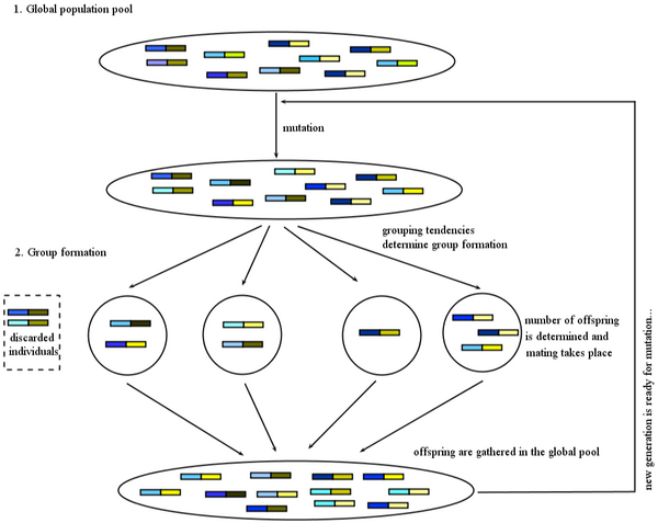
A central and shared feature of all simulation models encompassed in the program is that there are two distinct stages in a life cycle. At one stage, all individuals are gathered together without structure in a global population pool. At the other stage, individuals form groups, in which reproduction takes place. The transition of a population from the global pool to the groups, and the reproduction within the groups before the offspring returns to the global pool is where the simulation program offers different possibilities. Mutation takes place when individuals are in the global pool.
From the global pool to the groups
Individuals leave the global pool in random order. When they leave, they go to visit sites, where they either initiate new groups, or join already formed groups. If a site is empty, they join (initiate a new group) with probability 1. If a site is not empty, then the program offers two possibilities for the probability with which they join, from which the user can choose.
For the default option, the probability that individual i, that itself has grouping tendency gi, will join a group whose average grouping tendency of  is
is

The second option for the joining probability is called truncated joining in the computer program, and it truncates the possible group sizes at n * , and reduces the probability of joining more for larger groups than for smaller groups. Here the probability of joining a group that consists of n individuals is

for n < n * , where n * is the expected stable group size. The stable group size is the fixed point of the fitness function (see below), assuming that  . Whenever
  , the group acceptance probability is 0.
The second option matches the model in Avilés et al. (2002). Given a distribution of g’s in the population, the distribution of sizes will be somewhat different between the two. Also, if selection would produce the same average group size, the shape of the distribution of group sizes will differ a bit. Running the two options however shows that this does not really make a difference for the group size in the fixed point. Because the computation of n * requires information that individuals in realistic situations may not have, one can therefore, without changing the model results, resort to the first version that requires less information. The only advantage of the second, truncated version is that it gets to the fixed point faster.
The program allows for three options for the order in which the sites are visited. One option (called Random in the program) is that every individual visits the sites in random order. Another option (Forward) is that everyone starts at site number 1, then goes to site number 2, then to number 3 and so on. The third option (Backwards) is that everyone starts trying to be admitted at the non-empty site with the highest number. Say that this is site number n. Then it goes backwards, first to site n-1, then to n-2 and so on, until it is at site number 1. If the individual is then still not admitted, it starts a new group at site n+1.
These different orders of visiting will produce different size distributions; with Forward, the variance in sizes will be the largest, with Backwards it will be the smallest, and with Random it will be somewhere in between.
How many sites there will be and when the flow from the global population pool to the groups stops, depends on the way in which the size of the global population is balanced; there are three options (limited nesting sites, global density dependence, limited total population) that are discussed below.


