Price 2.0
From Evolution and Games
(→The Price equation for this slightly less simple model) |
(→The Price equation for this slightly less simple model) |
||
| Line 140: | Line 140: | ||
| - | As before, it is unfortunate that George Price named the term between square brackets in this equation | + | As before, it is unfortunate that George Price named the term between square brackets in this equation ''Cov(z,q)''. The claim of the Price equation - which we contend even more now - is that the equation unveils that a change in frequency - <math>\triangle Q</math> - is explained by the covariance between having the gene and the number of offspring - ''Cov(z,q)''. |
| - | of the Price equation - which we contend even more now - is that the equation unveils that a change in frequency - | + | |
| + | Two issues remain. One is that now there is another term on the right hand side. In the Price equation literature, this term tends to be crossed off, "because it will be 0 anyway". This is not correct; it is typically non-zero, even if it is 0 ''in expectation''. The other issue is that "''Cov( z,q)''" is still not a covariance; it is not a constant property of a random variable, but it is a random variable itself, as it differs from draw to draw. | ||
Revision as of 19:47, 18 September 2010
A model with sexual reproduction
If we add sexual reproduction, everything gets slightly more complicated, the proper statistics as well as the Price equation. This makes the statistics much more fun, and it makes the failure of the Price equation to be of any help even more salient. We like to keep it relatively simple though, so for the moment we do not assume actual different sexes, but we do assume that every individual is diploid. That means that individuals can be AA, Aa or aa. The frequency of the gene is then, resp., 1, 1/2 or 0. Individuals are hermaphrodites for the sake of simplicity.
Suppose that we have a population of 4 individuals, q1 = 1, q2 = q3 = 1 / 2 and q4 = 0. The next generation of 4 individuals is drawn as follows. First we draw a father for the first individual. From the father we draw one of the two loci, which gives us an A or an a. Then we draw a mother, and one of her loci. These two loci go into the gametes for reproduction, that together give us the first individual of the offspring generation. Three repetitions of this procedure give us a whole new generation.
We will make two crucial assumptions here.
1) A is not dominant nor recessive in fitness terms
2) Fair meosis
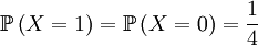
Both assumptions concern probabilities in this update step. The first concerns the probabilities with which an individual is chosen for parenthood. We assume that the probability with which individual i is chosen is
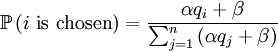
With our starting point, q1 = 1, q2 = q3 = 1 / 2 and q4 = 0. which gives us the following probabilities...
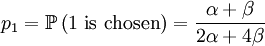
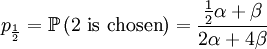

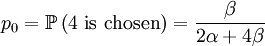
These formulas tells us that Assumption 1) is equivalent to saying that  is the average of p1 and p0. The second assumption just means that the probability of either locus of the parent to be chosen for passing on is 1/2.
Again, we first draw one of the individuals from the parent population (this is a hypothetical random variable that has nothing to do with the actual transition) and then draw the next generation (this is the actual random thing that happens in the the transition). The random variable X is again defined as the genotype of the parent. For our given starting point, that is
 and
and 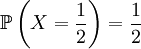 .
.
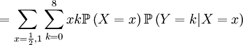
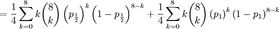
Then we define the random variable Y as the number of successful gametes that this parent produces. This is a slightly more omplicated random variable, because we need to draw 8 parents for 4 offspring and because the chances depend on which of the four the (candidate) parent is that was drawn in step 1. So we get a pretty long list of conditional probabilities.
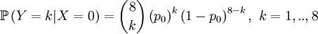

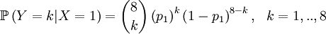
This is well defined again, so we can also compute the covariance of these two actual random variables. Let us start with expectations...
![\mathbb{E}\left[ X\right] =\frac{1}{2}](/wiki/images/math/0/b/d/0bd46ff59bf74b583131d663f920c02d.png)
![\mathbb{E}\left[ X\right] =\sum_{x=0,\frac{1}{2},1}x\mathbb{P}\left(X=x\right) =](/wiki/images/math/5/d/4/5d48b00bde13d310b2782f52ed3ee6f5.png)
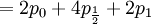
For symmetry reasons (the total number of succesful gametes is 8, and either of the 4 could be the parent)...
![\mathbb{E}\left[ Y\right] =2](/wiki/images/math/f/a/2/fa2e0acebdd016dff6fe97a86ea402ef.png)
![\mathbb{E}\left[ Y\right] = \sum_{x=0,\frac{1}{2},1}\sum_{y=0}^{8}y\mathbb{P}\left( X=x,Y=y\right) =](/wiki/images/math/5/a/3/5a339851c99ad6c8553b6f229f2dd79f.png)


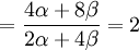
![\mathbb{E}\left[ XY\right] ==\frac{3\alpha +4\beta }{2\alpha +4\beta }](/wiki/images/math/f/b/c/fbc9e49e9cd1e8ccfffa158a2d19aae0.png) .
.
![\mathbb{E}\left[ XY\right] =\sum_{x=0,\frac{1}{2},1}\sum_{y=0}^{8}xy\mathbb{P}\left( X=x,Y=y\right) \text{ (because }xy=0\text{ if either }x=0\text{ or }y=0\text{)}](/wiki/images/math/d/2/7/d27b87768a6b6b0cb7bb0fa952113e7f.png)


The covariance of these two random variables is therefore...
![Cov\left( X,Y\right) =\mathbb{E}\left[ XY\right] -\mathbb{E}\left[ X\right] \mathbb{E}\left[ Y\right] =2\left( p_{\frac{1}{2}}+p_{1}\right) -1=\frac{3\alpha +4\beta }{2\alpha +4\beta }-1](/wiki/images/math/f/5/7/f572accbde31bc85b111e034f153ae6a.png)
The Price equation for this slightly less simple model
Interesting questions would be: is it good to have this gene? In this case, a first check in search of an answer would be:
is 
in other words, is α > 0, which, as long as we remain within the setting of this model, is equivalent to  . This however is only a first check, and below we will see that the answer can come in a riot of colours and flavours, especially if we are not really sure after all if the model describes reality accurately. But first we will look at what the Price equation makes of all this.
With this model, the Price equation looks pretty much like the one Price formulated in his original paper. It is an identity. The frequency of the gene in the parent population is, in general, defined as
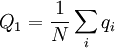
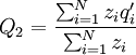
where N is the number of individuals, and qi is the frequency of the gene in individual i. So here that is Q1 = 1 / 2. The frequency of the gene in the offspring population is...
 .
.
This differs from the Price Equation 1.0, because of the locus-drawing step. Therefore we have $q_{i}^{\prime }$, which is the frequency of the gene in the set of successful gametes produced by individual i. In the [Price_1.0 | Price Equation 1.0] this was by definition equal to the frequency qi of the gene in the parent, but because there is a random step involved here, this is no longer the case. Of course zi is still the number of times individual i in the parent population was drawn for reproduction. The Price equation for this model is then is the following identity:
![\triangle Q=Q_{2}-Q_{1}=\frac{N}{\sum_{i}z_{i}}\left[ \frac{\sum_{i}z_{i}q_{i}}{N}-\left( \frac{\sum_{i}z_{i}}{N}\right) \left( \frac{\sum_{i}q_{i}}{N}\right) \right] +\frac{\sum_{i}z_{i}\left( q_{i}^{\prime}-q_{i}\right) }{\sum_{i}z_{i}}](/wiki/images/math/4/b/0/4b0c52a6045d8608aa987f4ed601e57f.png)
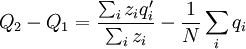
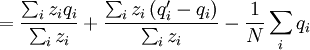

![=N\left[ \frac{\frac{1}{N}\sum_{i}z_{i}q_{i}-\left( \frac{1}{N}\sum_{i}z_{i}\right) \left( \frac{1}{N}\sum_{i}q_{i}\right) }{\sum_{i}z_{i}}\right] +\frac{\sum_{i}z_{i}\left( q_{i}^{\prime }-q_{i}\right) }{\sum_{i}z_{i}}](/wiki/images/math/9/5/d/95de4b8659ff773377c43f61dac3dd28.png)
![=\frac{N}{\sum_{i}z_{i}}\left[ \frac{\sum_{i}z_{i}q_{i}}{N}-\left( \frac{\sum_{i}z_{i}}{N}\right) \left( \frac{\sum_{i}q_{i}}{N}\right) \right] +\frac{\sum_{i}z_{i}\left( q_{i}^{\prime }-q_{i}\right) }{\sum_{i}z_{i}}](/wiki/images/math/3/9/c/39c0a7d8343290fcb3d8e4990805ed7e.png)
which in this particular model is
![\triangle Q=\frac{1}{2}\left[ \frac{\sum_{i}z_{i}q_{i}}{4}-\frac{\sum_{i}q_{i}}{2}\right] +\frac{\sum_{i}z_{i}\left( q_{i}^{\prime}-q_{i}\right) }{8}](/wiki/images/math/8/5/c/85c66ebfb6c0560dd17ba891f3d9e5cb.png)
As before, it is unfortunate that George Price named the term between square brackets in this equation Cov(z,q). The claim of the Price equation - which we contend even more now - is that the equation unveils that a change in frequency -  - is explained by the covariance between having the gene and the number of offspring - Cov(z,q).
Two issues remain. One is that now there is another term on the right hand side. In the Price equation literature, this term tends to be crossed off, "because it will be 0 anyway". This is not correct; it is typically non-zero, even if it is 0 in expectation. The other issue is that "Cov( z,q)" is still not a covariance; it is not a constant property of a random variable, but it is a random variable itself, as it differs from draw to draw.
