Price 2.0
From Evolution and Games
A model with sexual reproduction
If we add sexual reproduction, everything gets slightly more complicated, the proper statistics as well as the Price equation. This makes the statistics much more fun, and it makes the failure of the Price equation to be of any help even more salient. We like to keep it relatively simple though, so for the moment we do not assume actual different sexes, but we do assume that every individual is diploid. That means that individuals can be AA, Aa or aa. The frequency of the gene is then, resp., 1, 1/2 or 0. Individuals are hermaphrodites for the sake of simplicity.
Suppose that we have a population of 4 individuals, q1 = 1, q2 = q3 = 1 / 2 and q4 = 0. The next generation of 4 individuals is drawn as follows. First we draw a father for the first individual. From the father we draw one of the two loci, which gives us an A or an a. Then we draw a mother, and one of her loci. These two loci go into the gametes for reproduction, that together give us the first individual of the offspring generation. Three repetitions of this procedure give us a whole new generation.
We will make two crucial assumptions here.
1) A is not dominant nor recessive in fitness terms
2) Fair meosis
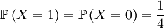
Both assumptions concern probabilities in this update step. The first concerns the probabilities with which an individual is chosen for parenthood. We assume that the probability with which individual i is chosen is
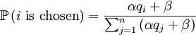
With our starting point, q1 = 1, q2 = q3 = 1 / 2 and q4 = 0. which gives us the following probabilities...
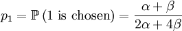
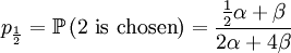

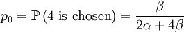
These formulas tells us that Assumption 1) is equivalent to saying that  is the average of p1 and p0. The second assumption just means that the probability of either locus of the parent to be chosen for passing on is 1/2.
Again, we first draw one of the individuals from the parent population (this is a hypothetical random variable that has nothing to do with the actual transition) and then draw the next generation (this is the actual random thing that happens in the the transition). The random variable X is again defined as the genotype of the parent. For our given starting point, that is
 and
and 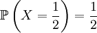 .
.
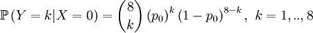
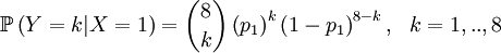
Then we define the random variable Y as the number of successful gametes that this parent produces. This is a slightly more omplicated random variable, because we need to draw 8 parents for 4 offspring and because the chances depend on which of the four the (candidate) parent is that was drawn in step 1. So we get a pretty long list of conditional probabilities.

This is well defined again, so we can also compute the covariance of these two actual random variables. Let us start with expectations...
