Repeated Games and Population Structure
From Evolution and Games
(→Lifecycle) |
(→Lifecycle) |
||
| Line 8: | Line 8: | ||
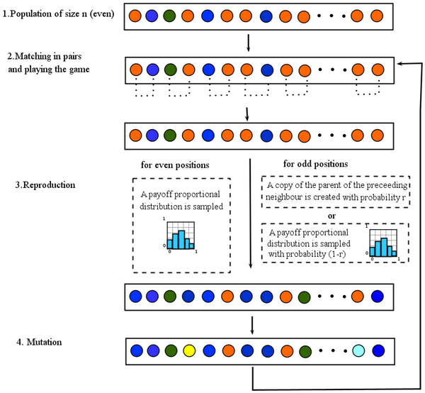
The following figure represents the lifecycle in the computer program. In '''step one''' we start with an even-sized population of finite state automata (initial population is made out of ALLD strategies). In '''step two''' individuals are matched in pairs to play the game - your are matched with your rightmost neighbor. The game is played between each pair of matched players, a one-shot game is played for sure and from then on the one-shot game is repeated with probability <math>\delta</math>. In '''step three''' reproduction takes place, a payoff proportional distribution is constructed. To fill up the next population we proceed in the following manner: with probability <math>1-r</math> the distribution is sampled, with probability <math>r</math> a copy of the parent of your left neighbor is created (this takes care of assortment). Finally, in '''step four''', every individual can mutate with a given probability. From then we go back to matching, and so on. | The following figure represents the lifecycle in the computer program. In '''step one''' we start with an even-sized population of finite state automata (initial population is made out of ALLD strategies). In '''step two''' individuals are matched in pairs to play the game - your are matched with your rightmost neighbor. The game is played between each pair of matched players, a one-shot game is played for sure and from then on the one-shot game is repeated with probability <math>\delta</math>. In '''step three''' reproduction takes place, a payoff proportional distribution is constructed. To fill up the next population we proceed in the following manner: with probability <math>1-r</math> the distribution is sampled, with probability <math>r</math> a copy of the parent of your left neighbor is created (this takes care of assortment). Finally, in '''step four''', every individual can mutate with a given probability. From then we go back to matching, and so on. | ||
| + | <center> | ||
[[File:RepeatedGamesAndPopulationStructureLifeCycle.png|600px|center|thumb|Lifecycle]] | [[File:RepeatedGamesAndPopulationStructureLifeCycle.png|600px|center|thumb|Lifecycle]] | ||
</center> | </center> | ||
Revision as of 14:04, 7 June 2010
Contents |
Run the simulations
You can download the software here. Once the program is running just click on the big play button to start the fun. Feel free to re-arrange and re-size the windows, zoom-in and out as the program is running. Click here if you need more information about running this program.
Lifecycle
The following figure represents the lifecycle in the computer program. In step one we start with an even-sized population of finite state automata (initial population is made out of ALLD strategies). In step two individuals are matched in pairs to play the game - your are matched with your rightmost neighbor. The game is played between each pair of matched players, a one-shot game is played for sure and from then on the one-shot game is repeated with probability δ. In step three reproduction takes place, a payoff proportional distribution is constructed. To fill up the next population we proceed in the following manner: with probability 1 − r the distribution is sampled, with probability r a copy of the parent of your left neighbor is created (this takes care of assortment). Finally, in step four, every individual can mutate with a given probability. From then we go back to matching, and so on.


