Repeated Games and Population Structure
From Evolution and Games
(→Strategies in the computer) |
(→Lifecycle) |
||
| Line 9: | Line 9: | ||
* In '''step one''' we start with an even-sized population of finite state automata (initial population is made out of ALLD strategies). | * In '''step one''' we start with an even-sized population of finite state automata (initial population is made out of ALLD strategies). | ||
| - | * In '''step two''' individuals are matched in pairs to play the game - your are matched with your rightmost neighbor. The game is played between each pair of matched players | + | * In '''step two''' individuals are matched in pairs to play the game - your are matched with your rightmost neighbor. The repeated game is played between each pair of matched players (one PD game is played for sure and from then on the game is repeated with probability <math>\delta</math>). |
| - | * In '''step three''' reproduction takes place, a payoff proportional distribution is constructed. To fill up the | + | * In '''step three''' reproduction takes place, a payoff proportional distribution is constructed. To fill up the population in the next generation we proceed in the following manner: the individuals in even positions (we start counting at 0) are determined by sampling from the probability distribution; for odd positions, with probability <math>r</math> a copy of the parent of your left neighbor is created, and with probability <math>1-r</math> an individual is sampled from the payoff proportional distribution (this takes care of assortment). |
* Finally, in '''step four''', every individual can mutate with a given probability. From then we go back to matching, and so on. | * Finally, in '''step four''', every individual can mutate with a given probability. From then we go back to matching, and so on. | ||
Revision as of 14:57, 7 June 2010
Contents |
Run the simulations
You can download the software here. Once the program is running just click on the big play button to start the fun. Feel free to re-arrange and re-size the windows, zoom-in and out as the program is running. Click here if you need more information about running this program.
Lifecycle
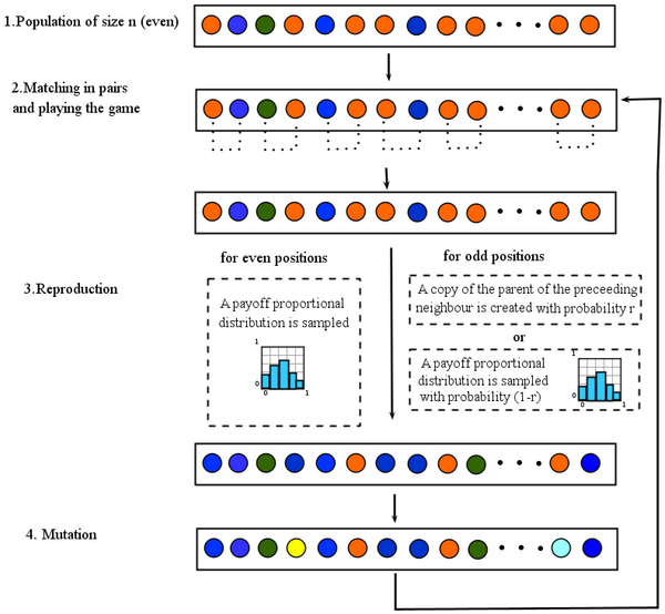
The following figure represents the lifecycle in the computer program.
- In step one we start with an even-sized population of finite state automata (initial population is made out of ALLD strategies).
- In step two individuals are matched in pairs to play the game - your are matched with your rightmost neighbor. The repeated game is played between each pair of matched players (one PD game is played for sure and from then on the game is repeated with probability δ).
- In step three reproduction takes place, a payoff proportional distribution is constructed. To fill up the population in the next generation we proceed in the following manner: the individuals in even positions (we start counting at 0) are determined by sampling from the probability distribution; for odd positions, with probability r a copy of the parent of your left neighbor is created, and with probability 1 − r an individual is sampled from the payoff proportional distribution (this takes care of assortment).
- Finally, in step four, every individual can mutate with a given probability. From then we go back to matching, and so on.
Strategies in the computer
Representation
Strategies are programmed explicitly as finite state automata(the program also has options for regular expressions, or Turing machines - see information onRepeated Games for more details about these additional representations).
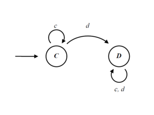
A finite automaton is a list of states, and for every state it prescribes what the automaton plays when in that state, to which state it goes if the opponent plays cooperate, and to which state it goes if the opponent plays defect.
The computer representation of the automate above is an array with the following values:
[(C, 0, 1) | (D, 1, 1)]
Each array position represents a state. The first state (indexed 0) codes the action for the empty game history, and the indexes of where to go if the opponent plays cooperation, and defection respectively. There is no limit on the size of this arrays that can grow and shrink dynamically as mutations produce new strategies.


